Introduction

Sparse regression is a useful technique to do variable selection, and achieve Bias-Variance trade-off. The lasso is a popular tool for sparse regression, especially for problems in which the number of variables \(p\) exceeds the number of observations \(n\).

To minimize a general loss penalized by the adaptive Lasso, we have developed a new algorithm Fabs, which is implemented in R package GFabs. Specifically, Fabs produces solutions for minimizing following objective function with a sequence of tuning \(\lambda\)， \[ L(\beta) + \lambda \sum_j w_j|\beta_j|, \] where \(w=(w_1, \dots, w_p)^\top\) is a vector of prefixed weights. Fabs can handle general loss functions, including both convex and nonconvex loss. It produces statistical guaranteed solutions (CSDA2018) with assumptions:

• \(L(\beta)\) to be differentiable, and

• \(\nabla^2 L\preceq M I\).

Here we provide a numeric example.

Nonconvex loss: high-dimensional smoothed partial rank estimator

The smoothed partial rank loss (Song et al. 2006) is an important nonconvex loss that not only includes the maximum rank loss (Han 1987) as its special case, but also accommodates general forms of censoring.

Consider a random sample of size \(n\). Let \(T_i\) be the outcome and \(C_i\) be the censoring variable of individual \(i\). Let \(X_i=(x_{i1},\dots, x_{ip})^\top\) be the vector of covariates for individual \(i\). The observed survival data consist of \((y_i, \delta_{i}, X_{i}), i = 1,2,\dots,n\), where \(y_i = \min\{T_i,C_i\}\) and \(\delta_{i} = I(T_{i} \leq C_{i})\).

The nonconvex SPR loss is a two-order U-statistics: \[ L(\beta) = -\frac{1}{n(n-1)} \sum_{i \neq i'}^n \delta_j I(y_i \geq y_{i'}) S_{\sigma}(X_i^\top\beta - X_{i'}^\top\beta), \]

set.seed(20132014)
N <- 400
p <- 50
nzc <- p/10
x <- matrix(rnorm(N * p), N, p)
beta = rnorm(nzc)
fx <- x[, seq(nzc)] %*% beta
hx <- exp(fx)
y <- rexp(N, hx)
tcens <- rbinom(n = N, prob = 0.3, size = 1)  # censoring indicator
status <- 1-tcens 

# Coordinate descent
library(glmnet)
## Loading required package: Matrix
## Loaded glmnet 4.1-7
library(survival)
fit <- glmnet(x, Surv(y, status), family = "cox")

# Fabs
group <- 1:p
library(GFabs)
fit_cox <- GFabs(x, y, group, status, model = "cox")
fit_spr <- GFabs(x, y, group, status, model = "spr")

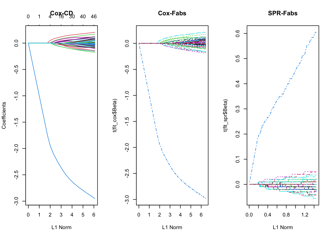
par(mfrow = c(1, 3))
plot(fit, main = "Cox-CD")
matplot(colSums(abs(fit_cox$Beta)), t(fit_cox$Beta), type = "l", main = "Cox-Fabs", xlab = "L1 Norm")
matplot(colSums(abs(fit_spr$Beta)), t(fit_spr$Beta), type = "l", main = "SPR-Fabs", xlab = "L1 Norm")